How to Unhide Rows in Google Sheets

To unhide rows in Google Sheets, simply select the hidden rows, right-click, and choose “Unhide rows.” Google Sheets is a powerful tool for creating and managing spreadsheets.

Sometimes, you may accidentally hide certain rows in your sheet and need to bring them back into view. Knowing how to unhide rows is essential for maintaining the clarity and organization of your data. In this guide, we will explore the step-by-step process of unhiding rows in Google Sheets, making it easy for you to manage your spreadsheet effectively.

Follow these instructions to effortlessly unhide rows in Google Sheets and streamline your data management process.

Credit: www.lifewire.com

Why Hide Rows?

When working with a large amount of data in Google Sheets, hiding rows can be a useful organizational tool. There are various reasons why you might want to hide rows in your spreadsheet, such as keeping your data organized and maintaining privacy. Let’s explore some of the common reasons under the subheadings of Organization and Privacy.

Organization

Hiding rows in Google Sheets can help you maintain a clean and organized spreadsheet. When you’re dealing with extensive data, hiding unnecessary rows can make it easier to focus on the important information. This feature is especially useful when working collaboratively on a shared spreadsheet, as it allows you to hide rows that may not be relevant to certain team members.

Privacy

Another key reason for hiding rows is to maintain the privacy of sensitive information. Whether you’re sharing a spreadsheet with others or simply want to keep certain data hidden from view, the ability to hide rows provides an added layer of privacy and control over who can access specific information.

By understanding why you might want to hide rows in Google Sheets, you can effectively utilize this feature to improve organization and privacy within your spreadsheets.

Credit: www.simplesheets.co

Hiding Rows In Google Sheets

Learn how to hide and unhide rows in Google Sheets to organize and manage your data with ease. These simple steps will help you manipulate your spreadsheet effectively.

Hiding Rows in Google Sheets Selecting Rows To hide rows in Google Sheets, start by selecting the specific rows you want to hide. Using the Menu Navigate to the “Format” menu. Click on “Row” and then select “Hide rows” to hide the selected rows. Using Keyboard Shortcuts For a quicker option, use the keyboard shortcut Ctrl + Shift + 9 to hide the selected rows in Google Sheets.

Unhiding Rows In Google Sheets

Unhiding Rows in Google Sheets is a simple process that allows you to display previously hidden rows in your spreadsheet.

Using The Menu

To unhide rows in Google Sheets using the menu, start by selecting the range of rows above and below the hidden rows.

1. Go to the “Format” menu.
2. Select “Rows” from the dropdown menu.
3. Click on “Unhide rows” to reveal the hidden rows.

Using Keyboard Shortcuts

If you prefer using keyboard shortcuts in Google Sheets, follow these steps:

1. Select the range of rows above and below the hidden rows.
2. Press Ctrl + Shift + 9 on Windows or Cmd + Shift + 9 on Mac.
3. The hidden rows will be unhid instantly.

Credit: www.simplesheets.co

Tips And Tricks

If you want to become a Google Sheets pro, you’ll need to master the knack of unhiding rows. Don’t worry! With a few tips and tricks, you’ll be navigating your Google Sheets like a pro in no time. Let’s explore some handy methods for unhiding rows and boosting your productivity.

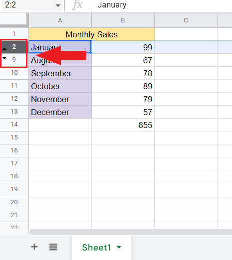
Grouping Rows

Grouping rows is a fantastic way to organize your data and simplify the process of unhiding multiple rows at once. To do this, simply select the rows you wish to group, right-click, and then choose “Group rows”. Once your rows are grouped, you can easily unhide them by clicking the small arrow that appears on the left side of your sheet when you hover over the grouped area.

Freezing Rows

Freezing rows can be a game-changer when it comes to navigating large datasets. By freezing rows at the top of your sheet, you can keep important headers in view no matter how far you scroll. To freeze rows, select the row below the last one you want to freeze, then go to “View” in the menu bar, select “Freeze”, and choose “Up to current row”. Voila! You can now unhide your frozen rows with ease.

Frequently Asked Questions Of How To Unhide Rows In Google Sheets

How Do I Unhide All Rows In Google Sheets?

To unhide all rows in Google Sheets, follow these steps. First, select any row by clicking on the row number. Then, press Ctrl + Shift + 9 on Windows or Command + Shift + 9 on Mac. This will unhide all hidden rows in your spreadsheet.

How Do I Unhide Hidden Rows?

To unhide hidden rows, select the rows adjacent to the hidden ones, right-click, and choose “Unhide. ” Alternatively, navigate to the “Home” tab, click on “Format,” and select “Unhide Rows. “

Why Are Rows Missing On My Google Sheet?

Rows may be hidden or filtered. Ensure there are no applied filters or manual hiding.

How Do I Make Rows Always Visible In Google Sheets?

To make rows always visible in Google Sheets, freeze the rows by selecting the row(s), then go to View > Freeze > 1 row.

Conclusion

Knowing how to unhide rows in Google Sheets can significantly enhance your productivity when working with large datasets. By following the simple steps outlined in this guide, you’ll be equipped to effortlessly manage and organize your data effectively. Now, with this newfound skill, you can work more efficiently and tackle your projects with ease.