To cross out a cell in Excel, simply select the cell and press the “Strikethrough” button in the Home tab. This will put a line through the content.
Excel provides various formatting options to help you visually organize and manipulate your data. One of these options is the ability to cross out cells, which can be useful for indicating completed tasks or marking off items from a list.
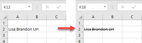
By using the “Strikethrough” feature in Excel, you can easily draw attention to specific cells without having to delete the contents entirely. We will explore how to cross out a cell in Excel and discuss the benefits of using this formatting technique in your spreadsheets.
Credit: excelspreadsheetshelp.blogspot.com
How To Cross Out A Cell In Excel
Crossing out a cell in Excel can be a useful way to visually represent deleted or outdated information. Whether you’re working on a list, table, or any other type of Excel sheet, there are a couple of methods you can use to achieve this. In this guide, we’ll walk you through how to cross out a cell in Excel using two different approaches.
Using Strike-through Formatting
One simple way to cross out a cell in Excel is by utilizing the strike-through formatting feature. Follow these steps to apply this formatting:
- Select the cell you want to cross out
- Navigate to the Home tab in the Excel menu
- Locate the Font section
- Click on the B (Bold) button to reveal the formatting options
- Click on the abc with a strikethrough icon
- The selected cell will now display with a strikethrough effect
Using Conditional Formatting
Another method for crossing out a cell involves using conditional formatting. This approach is particularly useful for automating the process based on specific criteria. Follow these steps to apply conditional formatting:
- Select the cell or range of cells you want to apply the strikethrough effect to
- Navigate to the Home tab in the Excel menu
- Click on Conditional Formatting in the Styles group
- Select New Rule to open the New Formatting Rule dialog box
- Choose Use a formula to determine which cells to format
- Enter the formula to determine the conditions for the strikethrough effect
- Click Format and select Font to apply strikethrough formatting
- Click OK to apply the conditional formatting rule
Credit: www.ablebits.com
Tips And Tricks
Excel Cross Out Cell feature offers a handy way to visually denote certain information. When it comes to mastering this function, here are some essential tips and tricks to maximize your efficiency:
Crossing Out Multiple Cells
To cross out multiple cells simultaneously:
- Select the range of cells you want to cross out.
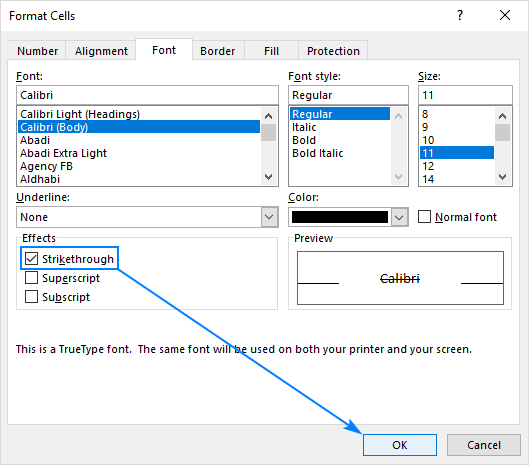
- Right-click on the selection and choose ‘Format Cells’.
- Go to the ‘Font’ tab and check the ‘Strikethrough’ option.
- Click ‘OK’ to apply the cross out formatting to the selected cells.
Removing The Cross Out Formatting
To remove the cross out formatting from cells:
- Highlight the cells with the strikethrough effect.
- Right-click on the selection and select ‘Format Cells’.
- Uncheck the ‘Strikethrough’ option under the ‘Font’ tab.
- Click ‘OK’ to remove the cross out formatting.
Credit: www.automateexcel.com
Frequently Asked Questions Of Excel Cross Out Cell
Is There A Way To Cross Out A Cell In Excel?
Yes, you can cross out a cell in Excel by selecting the cell and clicking the “Strike Through” button in the toolbar.
What Is Shortcut For Strikethrough In Excel?
To use the strikethrough shortcut in Excel, press “Ctrl” + “5”. This will apply the strikethrough formatting to the selected text or cell. Strikethrough is a useful way to visually indicate that data has been changed or is no longer relevant in your spreadsheet.
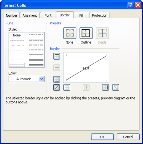
How Do You Cross A Diagonal Cell In Excel?
To cross a diagonal cell in Excel, you can use the “slash” (/) symbol as a separator in the formula. For example, to cross cell A1 with B2, you would enter the formula “=A1/B2”.
How Do You Cross Hatch A Cell In Excel?
To cross hatch a cell in Excel, select the cell(s) you want to format. Then, go to the “Home” tab, click on the “Fill” button in the “Font” group, and choose “More Colors. ” In the “Patterns” tab, select the desired pattern, such as diagonal lines.
Conclusion
Excel’s cross out cell feature is a valuable tool for visually marking data. It helps to streamline information organization and analysis. By utilizing this function effectively, users can enhance clarity and efficiency in their spreadsheets. This simple yet powerful feature can greatly improve the usability and visual appeal of Excel documents.